Deep Learning cheatsheet

Neural Networks

Neural networks are a class of models that are built with layers. Commonly used types of neural networks include convolutional and recurrent neural networks.

Architecture ― The vocabulary around neural networks architectures is described in the figure below:

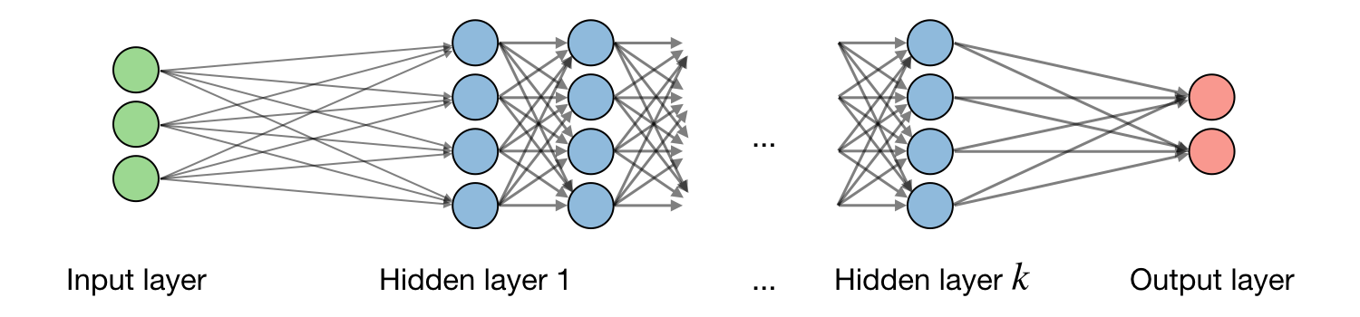
By noting $i$ the $i^{th}$ layer of the network and $j$ the $j^{th}$ hidden unit of the layer, we have:

$$z_j^{\left[i\right]}={w_j^{\left[i\right]}}^{T}x+b_j^{\left[i\right]}$$

where we note $w$, $b$, $z$ the weight, bias and output respectively.

Activation function ― Activation functions are used at the end of a hidden unit to introduce non-linear complexities to the model. Here are the most common ones:

Sigmoid	Tanh	ReLU	Leaky ReLU
$g\left(z\right)=\frac{1}{1+e^{-z}}$	$g\left(z\right)=\frac{e^z-e^{-z}}{e^z+e^{-z}}$	$g\left(z\right)=\text{max}(0,z)$	$g\left(z\right)=\text{max}(ϵz,z)$ with $ϵ\ll 1$

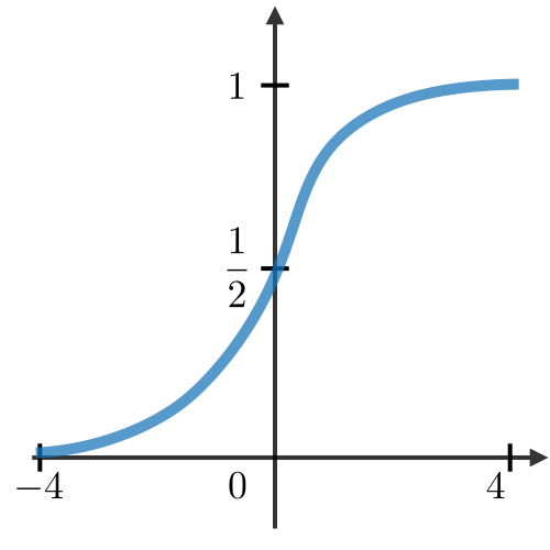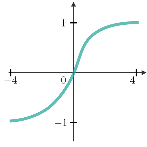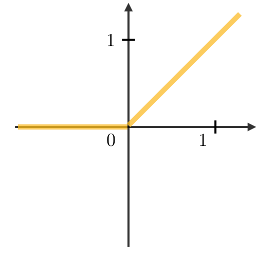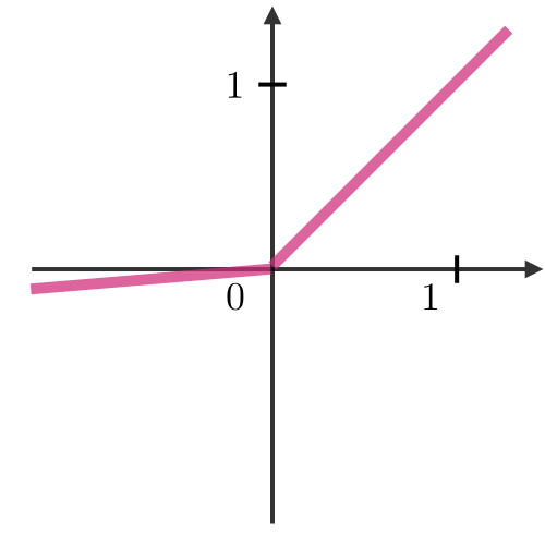Cross-entropy loss ― In the context of neural networks, the cross-entropy loss $L(z,y)$ is commonly used and is defined as follows:

$$L(z,y)=-[y\log \left(z\right)+(1-y)\log (1-z)]$$

Learning rate ― The learning rate, often noted $\alpha$ or sometimes $\eta$, indicates at which pace the weights get updated. This can be fixed or adaptively changed. The current most popular method is called Adam, which is a method that adapts the learning rate.

Backpropagation ― Backpropagation is a method to update the weights in the neural network by taking into account the actual output and the desired output. The derivative with respect to weight $w$ is computed using chain rule and is of the following form:

$$\frac{\partial L(z,y)}{\partial w}=\frac{\partial L(z,y)}{\partial a}\times \frac{\partial a}{\partial z}\times \frac{\partial z}{\partial w}$$

As a result, the weight is updated as follows:

$$w⟵w-\alpha \frac{\partial L(z,y)}{\partial w}$$

Updating weights ― In a neural network, weights are updated as follows:

• Step 1: Take a batch of training data.
• Step 2: Perform forward propagation to obtain the corresponding loss.
• Step 3: Backpropagate the loss to get the gradients.
• Step 4: Use the gradients to update the weights of the network.

Dropout ― Dropout is a technique meant at preventing overfitting the training data by dropping out units in a neural network. In practice, neurons are either dropped with probability $p$ or kept with probability $1-p.$

Convolutional Neural Networks

Convolutional layer requirement ― By noting $W$ the input volume size, $F$ the size of the convolutional layer neurons, $P$ the amount of zero padding, then the number of neurons $N$ that fit in a given volume is such that:

$$N=\frac{W-F+2P}{S}+1$$

Batch normalization ― It is a step of hyperparameter $\gamma ,\beta$ that normalizes the batch $\left\{x_i\right\}$. By noting ${\mu }_B,{\sigma }_B^2$ the mean and variance of that we want to correct to the batch, it is done as follows:

$$x_i⟵\gamma \frac{x_i-{\mu }_B}{\sqrt{{\sigma }_B^2+ϵ}}+\beta$$

It is usually done after a fully connected/convolutional layer and before a non-linearity layer and aims at allowing higher learning rates and reducing the strong dependence on initialization.

Recurrent Neural Networks

Types of gates ― Here are the different types of gates that we encounter in a typical recurrent neural network:

Input gate	Forget gate	Gate	Output gate
Write to cell or not?	Erase a cell or not?	How much to write to cell?	How much to reveal cell?

LSTM ― A long short-term memory (LSTM) network is a type of RNN model that avoids the vanishing gradient problem by adding 'forget' gates.

For a more detailed overview of the concepts above, check out the Deep Learning cheatsheets!

Reinforcement Learning and Control

The goal of reinforcement learning is for an agent to learn how to evolve in an environment.

Definitions

Markov decision processes ― A Markov decision process (MDP) is a 5-tuple $(S,A,\{P_{sa}\},\gamma ,R)$ where:

• $S$ is the set of states
• $A$ is the set of actions
• $\left\{P_{sa}\right\}$ are the state transition probabilities for $s\in S$ and $a\in A$
• $\gamma \in [0,1[$ is the discount factor
• $R:S\times A⟶R$ or $R:S⟶R$ is the reward function that the algorithm wants to maximize

Policy ― A policy $\pi$ is a function $\pi :S⟶A$ that maps states to actions.

Remark: we say that we execute a given policy $\pi$ if given a state $s$ we take the action $a=\pi \left(s\right)$.

Value function ― For a given policy $\pi$ and a given state $s$, we define the value function $V^{\pi }$ as follows:

$$V^{\pi }\left(s\right)=E[R\left(s_0\right)+\gamma R\left(s_1\right)+{\gamma }^{2}R\left(s_2\right)+...|s_0=s,\pi ]$$

Bellman equation ― The optimal Bellman equations characterizes the value function $V^{{\pi }^{\ast }}$ of the optimal policy ${\pi }^{\ast }$:

$$V^{{\pi }^{\ast }}\left(s\right)=R\left(s\right)+\underset{a\in A}{max}\gamma \sum _{s^{\prime }\in S}{P}_{sa}\left(s^{\prime }\right)V^{{\pi }^{\ast }}\left(s^{\prime }\right)$$

Remark: we note that the optimal policy ${\pi }^{\ast }$ for a given state $s$ is such that:

$${\pi }^{\ast }\left(s\right)=\underset{a\in A}{\text{argmax}}\sum _{s^{\prime }\in S}{P}_{sa}\left(s^{\prime }\right)V^{\ast }\left(s^{\prime }\right)$$

Value iteration algorithm ― The value iteration algorithm is in two steps:

1) We initialize the value:

$$V_0\left(s\right)=0$$

2) We iterate the value based on the values before:

$$V_{i+1}\left(s\right)=R\left(s\right)+\underset{a\in A}{max}\left[\sum _{s^{\prime }\in S}\gamma P_{sa}\left(s^{\prime }\right)V_i\left(s^{\prime }\right)\right]$$

Maximum likelihood estimate ― The maximum likelihood estimates for the state transition probabilities are as follows:

$$P_{sa}\left(s^{\prime }\right)=\frac{\#\text{times took action}a\text{in state}s\text{and got to}{s}^{\prime }}{\#\text{times took action}a\text{in state}s}$$

Q-learning ― $Q$-learning is a model-free estimation of $Q$, which is done as follows:

$$Q(s,a)\leftarrow Q(s,a)+\alpha [R(s,a,s^{\prime })+\gamma \underset{a^{\prime }}{max}Q(s^{\prime },a^{\prime })-Q(s,a)]$$